Convert Excel spreadsheet to OLSTF

Start point

It is expected that you have a list of values that can be read in Excel, such as:

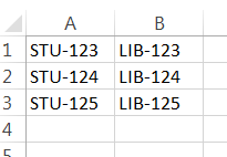
These values are presumed to represent the Secondary Code as the identifier from the Student record system and the Library Barcode. One Student per row. The values in these source columns need not change. This will be useful later.

Tag the data

The first stage is to assign the OLSTF tags to the data values. This can be done with a simple concatenation:

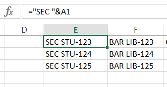
To enter this formula, click in the cell where the result should be placed. In this case “E1”. Once this cell is selected, click in the formula bar at the top, just after   and type the text as shown above. The above formula will place the “SEC” tag, followed by a space before the value from cell A1.

With the cursor in the top cell (E1) click the "handle" in the bottom right corner and drag this down the column to populate with concatenated values for all your data in column A.                                                                                                                                                                                     

Add default values

The next stage of the process is to determine some default tags and values to add to each record. These need only be added to a single cell each.

In this example the default User Category code of WTHD is specified.

Why not transpose the data using Copy/Paste?

 Caution: we recommend you don’t do this. Here we explain why.

There is a simple Copy/Paste process to carry out a Transpose action, but this does not deliver a useful next stage of the process. For example if we transpose A1-3, B1-3, we get:

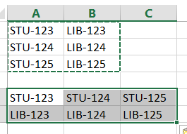
We therefore arrive at one student per column, which isn’t helpful.

Transpose the data using formulae

In order to generate the data needed, the source cell needs to be calculated.

To this end, you need to know how many lines are required for each record:

• The number of data values per student plus
• The number of default values plus
• 1 (the “end of record” line)

In the example here there are 2 data values and one default, giving 4 lines per record.

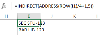
Starting in a new cell in your spreadsheet, the formula for the first line of each record will therefore be:

You can copy and paste the following to ensure that you have the syntax correct.
However, please note that the values will need to be amended as necessary.

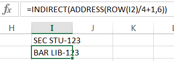
=INDIRECT(ADDRESS(ROW(I1)/4+1,5))

This breaks down to:

INDIRECT
Retrieve the value from a cell when given the ADDRESS

ADDRESS
Construct a cell address from the row and column numbers

ROW(I1)
The row number for the cell given.
Do not just put “1” here – see below

/4+1
There are four lines per record. For rows 1 to 3, we need to refer to student number 1. Excel will divide the current row number by 4, add 1 and ignore the decimal places. Thus: 1.25, 1.5 and 1.75 will all be treated as a reference to row number 1.

5
The first line’s value should come from the first column containing the tagged data in this case number 5 (Column E)

The formula for the second line of each record will therefore be:

This differs from the first line formula as follows:

ROW(I2)
The row number for the cell given.
This is now “I2” because this is cell “I2”
Thus “ 2/4+1 “ will still result in a reference to student number 1

6
The second line’s value should come from the second column containing the tagged data, in this case number 6 (Column F)

The third line is a simple copy of the default value:

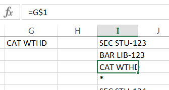
Note the “$” symbol, indicating that when this cell is copied to a subsequent row it should still get its value from row 1.

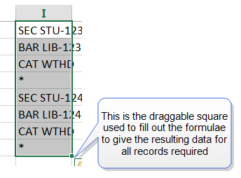
The fourth, the last line per record, is simply “*” – just enter this into the cell.

Copy the formulae to generate the data

Select all of the lines for the first record (ie: cells I1 through I4) and copy them to cell I5. Excel will fill I5 through I8. This will allow the reader to verify that the formula are operating correctly.

Note the number of rows for which you have data and multiply this by the number of lines per record.

Select all 8 cells and extend the formulae using the draggable square which shows on the bottom right of the selection border – dragging this all the way to the row for the last line of the file, as noted by multiplying the data rows by the lines per record.

At this stage it would be good practice to verify a selection of records to confirm that they contain the correct values.

Create the OLSTF file

Copy only the column that has just been extended to generate the data (eg: Column I) and paste it into Notepad. This can then be saved and imported into OLIB as a User Import file.

Reuse the spreadsheet

It should be simple to paste in updated data into the data columns (A and B) from fresh information supplied. It will therefore save the reader time for the next set of data to save this spreadsheet (with formulae). Note that if the original file was a .csv file from which this has been generated, then it will need to be saved as an Excel spreadsheet in order to preserve the formulae.

Also note that if there is a different number of source records, then the generated data column will need to be adjusted accordingly. This can be extended by selecting all of the lines for the whole of the last record before dragging the square to extend the results. If there are fewer records, then it is a simple matter to only copy fewer rows from this column into Notepad.

Automate the process

Converting your data from a csv file ready for import into OLIB can be automated and configured to take place during daystart. OCLC can implement this as minor chargeable work.

Other default values

If the intention is to prevent Users from borrowing more materials, then there are other methods of achieving this, depending on the OLIB Circulation configuration.

CIRCBAN Y
To present a “This User is Banned” message at the issue desk
Note that the User Import will not automatically unban a user with “CIRCBAN N”. Contact OCLC if this is contrary to requirement.

EXP 01-JUL-2015
To amend the User’s membership expiry so that loans are not issued beyond this date without overriding at the issue desk

Other potential defaults might be to change their location, department or other elements of the User’s record.

My spreadsheet has headings

If the spreadsheet has heading rows, then continue as if the heading row is the first record. You need not, however, copy that record into Notepad.